\(\newcommand{vrt}[2]{\left ( \begin{array}{l} #1 \\ #2 \end{array} \right )}\) \(\newcommand{defeq}{\overset{\mathit{def}}{=}}\) \(\newcommand{am}{\text{a.m.}}\) \(\newcommand{pm}{\text{p.m.}}\)

Overview

This post is a continuation of Towards a Mathematical Model of Computer Games. Unlike that post, this one is focused on mathematical rigor rather than motivation. Rather than defining a mathematical model of a MegaZeux game, it pursues the less ambitious goal of defining a mathematical model of tic-tac-toe. The game tic-tac-toe shares some common characteristics with a MegaZeux game.

The game involves two players. Each of these players is analogous to a MegaZeux robot, and the game board plays the role of the environment. The players repeatedly make requests to the board to alter its state. The board may or may not honor those requests depending on whether they obey its “laws of physics”.

The two players together with their environment will form a closed system, i.e. a set \(\mathit{GameState}\) with an update function

Or equivalently, a set of two functions, using \(1 = \{ \ast \}\) as both the input and output sets:

and

We will construct this closed system out of open systems such as the players. The players are open systems that take observations of the board state as inputs and produce move choices as outputs. As a rough first approximation, a player can be diagrammed as follows:

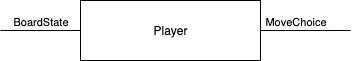
The above system is considered open because its input and output are not one-element sets; they contain actual information that must be received from and sent to unspecified destinations. Each turn, an element of BoardState is received as input. The player uses the current board state, possibly along with the player’s own internal state, to decide a move to submit to the board.

Now, let’s develop a formalism that allows us to compose complex systems from simpler systems.

Lenses

We model open systems mathematically using a construct called lenses. I learned about lenses from Categorical Systems Theory, which I highly recommend. In the interest of self-containment, I will rehash the fundamentals of lenses now.

Definitions

Definition

An arena \(\vrt{A^-}{A^+}\) is a pair consisting of two sets \(A^-\) and \(A^+\).

Definition

A lens \(\vrt{f^\sharp}{f} : \vrt{A^-}{A^+} \leftrightarrows \vrt{B^-}{B^+}\) is a pair consisting of two functions:

• A passforward function \(f : A^+ \to B^+\)
• A passback function \(f^\sharp : A^+ \times B^- \to A^-\)

The arena \(\vrt{A^-}{A^+}\) is called the domain of \(\vrt{f^\sharp}{f}\) and the arena \(\vrt{B^-}{B^+}\) is called the codomain of \(\vrt{f^\sharp}{f}\).

The passforward function of a lens can be viewed as sending information “downstream” and the passback function can be viewed as sending information “upstream”. One particularly important type of lens is a discrete dynamical system.

Definition

A discrete dynamical system (or dynamical system for short) is a lens of the form

\[\vrt{\mathit{nextState}}{\mathit{output}} : \vrt{\mathit{State}}{\mathit{State}} \leftrightarrows \vrt{\mathit{In}}{\mathit{Out}}\]

That is, a dynamical system is a lens whose domain is an arena of the form \(\vrt{\mathit{State}}{\mathit{State}}\) for some set \(\mathit{State}\).

Above, we consider \(\mathit{State}\) the type of our dynamical system’s internal state, \(\mathit{In}\) the type of its input, and \(\mathit{Out}\) the type of its output. Expanding the definition of lens, we see that

• \(\mathit{nextState} : \mathit{State} \times \mathit{In} \to \mathit{State}\) is a function that takes a pair of a “current” state and an input to a “next” state.
• \(\mathit{output} : \mathit{State} \to \mathit{Out}\) is a function that takes a state to an output.

This matches the intuitive structure of game engines that I presented previously. Those familiar with digital logic may know the distinction between Moore machines and Mealy machines. The output of a Mealy machine may depend both on its input and its current state, whereas the output of a Moore machine may only depend on its current state. In this sense, a dynamical system is like a Moore machine rather than a Mealy machine: before its input can affect its output, it must store the input in its state as an intermediate step. This can be a bit awkward sometimes, but it’s not a fundamental problem.

A dynamical system \(S : \vrt{\mathit{State}_S}{\mathit{State}_S} \leftrightarrows \vrt{\mathit{In}_S}{\mathit{Out}_S}\) can be depicted as follows.

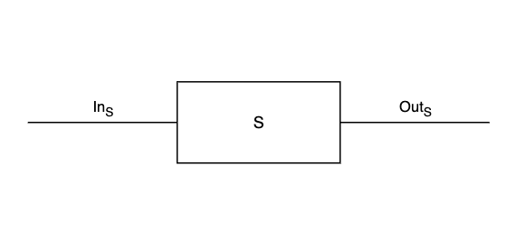
Note that the set \(\mathit{State}_S\) does not appear in the diagram, because it does not affect the systems that \(S\) interacts with.

If the codomain of one lens matches the domain of another then we can compose them together.

Definition

Given lenses \(\vrt{f^\sharp}{f} : \vrt{A^-}{A^+} \leftrightarrows \vrt{B^-}{B^+}\) and \(\vrt{g^\sharp}{g} : \vrt{B^-}{B^+} \leftrightarrows \vrt{C^-}{C^+}\) their composite \(\vrt{g^\sharp}{g} \circ \vrt{f^{\sharp}}{f}\) is defined as \(\vrt{h^\sharp}{h}\), where

• \(h\) is defined as the function composite \(g \circ f\)
• \(h^\sharp\) is defined such that \(h^\sharp(a^+, c^-) \defeq f^\sharp(a^+, g^\sharp(f(a^+), c^-))\)

We also have a parallel composition operator on lenses.

Definition

Given two lenses \(\vrt{f^\sharp}{f} : \vrt{A^-}{A^+} \leftrightarrows \vrt{B^-}{B^+}\) and \(\vrt{g^\sharp}{g} : \vrt{C^-}{C^+} \leftrightarrows \vrt{D^-}{D^+}\) we define their parallel product \(\vrt{f^\sharp}{f} \otimes \vrt{g^\sharp}{g} : \vrt{A^- \times C^-}{A^+ \times C^+} \leftrightarrows \vrt{B^- \times D^-}{B^+ \times D^+}\) is defined as the lens \(\vrt{h^\sharp}{h}\), where

\[h(a^+, c^+) \defeq (f(a^+), g(c^+))\]

and

\[h^\sharp(a^+, c^+, b^-, d^-) \defeq (f^\sharp(a^+, b^-), g^\sharp(c^+, d^-))\]

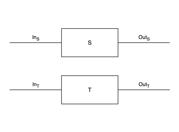
Given dynamical systems

and

their parallel product

can be depicted by juxtaposing the two dynamical systems.

Example

Here is an example of a dynamical system from Categorical Dynamical Systems. Define the set

We define a dynamical system

where \(f\) is the identity function

and

This system represents a wall clock, which takes no external input and advances one hour forward at each step.

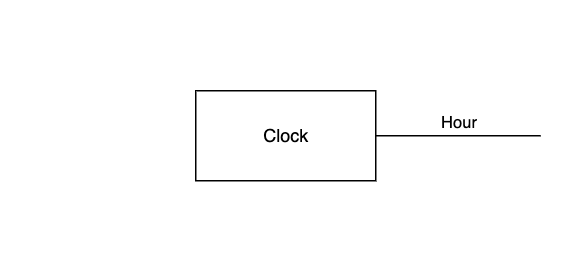
Note that we don’t need to draw an incoming edge; because the input is \(1 = \{ \ast \}\), it transmits only one possible choice of value \(\ast\). So instead of receiving input from an external source, \(\mathit{Clock}\) can fabricate the value \(\ast\) at every step, knowing it is the correct choice.

The above clock does not distinguish between \(\am\) and \(\pm\) To fix this, we define a dynamical system called \(Meridiem\) that shifts between \(\am\) and \(\pm\) We first define the set \(\am/\pm \defeq \{ \am, \pm \}\) Then we define

where

and

Now we need “wire together” the \(\mathit{Clock}\) and \(\mathit{Meridiem}\) systems. As a first step, we take their paralell product.

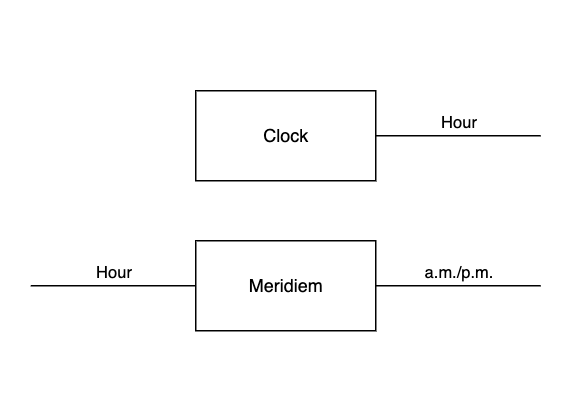
To feed the output of \(\mathit{Clock}\) into \(\mathit{Meridiem}\), we use composition, which can be depicted as nesting.

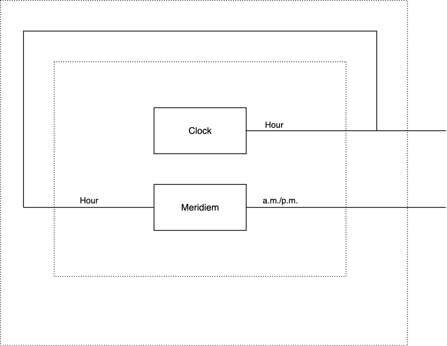
The inner dotted box is the parallel product \(\mathit{Clock} \otimes \mathit{Meridiem}\). The outer dotted box is the fully wired system. The section between the two boxes depicts a new lens

defined such that

and

The fully wired system, which we shall call \(\mathit{Clock}'\) is then defined as

Combinational Systems

Suppose that we want to translate the output of the \(\mathit{Clock}'\) system above to 24-hour time, also known as “military time”, instead of \(\am/\pm\) Let

We need to “post-compose” a function \(f : \mathit{Hour} \times \am/\pm \to \mathit{Hour24}\) after the \(\mathit{Clock}'\) system, where \(f\) is defined as follows:

Such a post-composition is depicted below

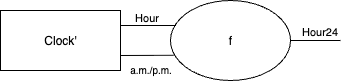
Note that \(f\) is just a function, not a dynamical system with state.

In digital logic, a circuit that stores state is known as sequential, whereas a circuit that merely computes a function is called combinational. The function \(f\) above, having no internal state, is combinational. We can post-compose a dynamical system by a combinational system using lens combination.

Without loss of generality, let \(\mathit{Out}_0 \defeq \mathit{Hour} \times \am/\pm\), let \(\mathit{Out}_1 \defeq \mathit{Hour24}\), and let \(\mathit{In} \defeq 1\). Then this lens should translate the system’s output using a function \(f : \mathit{Out}_0 \to \mathit{Out}_1\) but leave the input \(\mathit{In}\) unchanged. Hence we define it as

where \(\pi_1 : \mathit{Out_0} \times \mathit{In} \to \mathit{In}\) is the projection of the second component \((o,i) \mapsto i\).

We then obtain our military time clock as

Demultiplexors

Imagine a turn-based board game with multiple players. At each turn, we want to provide exactly one player with the state of the board so that they can make an informed move. The challenge is to send a payload value along a different wire depending on some selector value, and to send “nothing” along all other wires. More precisely, we need a combinational circuit, called a demultiplexor, that takes two inputs

• The payload, whose type \(\mathit{Payload}\) may vary
• The selector of type n + 1, deciding which, if any, of \(n\) output destinations to transmit the payload to

The demultiplexor circuit has \(n\) different output wires. Their type is not quite \(\mathit{Payload}\); each wire may contain a value of type \(\mathit{Payload}\) or, if it has not been selected, it may contain “no information” of type \(1\).

To express the set of values that each belong to exactly one of the disjoint sets \(\mathit{Payload}\) or \(1\) we need to use a set theoretic operation called the sum, which is not as well known as its evil twin the Cartesian product.

Definition Given sets \(X\) and \(Y\), their sum \(X + Y\) is defined as

\[X + Y \defeq \{ (0,x) \mid x \in X \} \cup \{ (1,y) \mid y \in Y \}\]

By tagging values with either \(0\) or \(1\), we ensure that the elements of the two operands are treated as mutually exclusive. It may be instructive to compare the set \(1 = 1 \cup 1\) with the set \(1 + 1\).

While we’re at it, let’s define another set-theoretic operation.

Definition Given sets \(X\) and \(Y\), \(X^Y\) is defined as the set of functions from \(Y\) to \(X\). In other words, \(X^Y\) is a synonym for \(Y \to X\).

Now we are ready to formally define the notion of demultiplexor circuits.

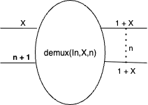
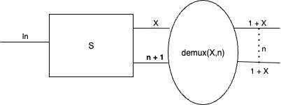
Definition The demultiplexor \(\mathit{demux}(\mathit{In}, X, n)\) is the combinational lens

\[\vrt{\pi_1}{f} : \vrt{\mathit{In}}{X \times (\mathbf{n + 1})} \leftrightarrows \vrt{\mathit{In}}{(1 + X)^\mathbf{n}}\]

where \(f : X \times (\mathbf{n + 1}) \to (1 + X)^\mathbf{n}\) is defined such that

\[f(x, m)(k) \defeq \begin{cases} (1,x) & \text{ if } m = k \\ (0,\ast) & \text{ if } m \neq k \end{cases}\]

and \(\pi_1 : (X \times (\mathbf{n + 1})) \times \mathit{In} \to \mathit{In}\) is the second projection function

\[\pi_1((x, m), i) \defeq i\]

Thus, the demultiplexor \(\mathit{demux}(\mathit{In}, X,n)\) allows us to either

• Select some \(m \in \mathbf{n}\) such that \((1,x)\) is transmitted along the \(m^{\mathit{th}}\) output wire and \((0,\ast)\) is transmitted along all other output wires.
• Or, if \(m = n\), then transmit \((0,\ast)\) along all wires.

\(\mathit{demux}(\mathit{In}, X,n)\) is depicted below, where we’ve elided all but the first and last of the \(n\) output wires.

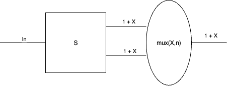
Note that \(\mathit{demux}(\mathit{In}, X, n)\) can only be post-composed with a dynamical system whose input set is \(\mathit{In}\). When a demultiplexor is post-composed with a system \(S : \vrt{\mathit{State}_S}{\mathit{State}_S} \leftrightarrows \vrt{\mathit{In}_S}{\mathit{Out}_S}\), we elide the \(\mathit{In}\) argument from \(\mathit{demux}\), instead inferring from context that \(\mathit{In} = \mathit{In}_S\):

Multiplexors

Assume \(n\) inputs of type \((1 + X)\), and further assume that we expect at most one input to have the form \((1, x)\) while the others have the form \((0,\ast)\). We want a combinational lens that produces a single output of type \(1 + X\), and which forwards \((1,x)\) if a single input has the form \((1,x)\) and forwards \((0,x)\) otherwise.

Definition The multiplexor \(\mathit{mux}(\mathit{In}, X, n)\) is the combinational lens

\[\vrt{\pi_1}{f} : \vrt{\mathit{In}}{(1 + X)^\mathbf{n}} \leftrightarrows \vrt{\mathit{In}}{1 + X}\]

where \(f : (1 + X)^\mathbf{n} \to (1 + X)\) is defined as

\[f(\phi) \defeq \begin{cases} \phi(m) & \text{if there exists a unique } m \in \mathbf{n} \text{ such that } \phi(m) = (1, x) \text{ for some } x \\ (0,\ast) & \text{otherwise} \end{cases}\]

and \(\pi_1 : (1 + X)^\mathbf{n} \times \mathit{In} \to \mathit{In}\) is the second projection function

\[\pi_1(\phi, i) \defeq i\]

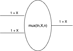
Similar to \(\mathit{demux}\), we typically infer the \(\mathit{In}\) argument.

Tic-tac-toe

Now we use the dynamical system techniques described above to model the game of tic-tac-toe. We do not model any notion of a winning condition, but instead focus on the evolution of the game over time, where two agents (players) influence the environment (the board) by submitting moves in a turn-based fashion.

Overview

To model the board, we first need a notion of cell locations. Let each bold natural number \(\mathbf{n}\) denote the set of natural numbers less than it, i.e. \(\mathbf{n} \defeq \{ 0, 1, \ldots, n-1 \}\). A location on a tic-tac-toe board consists of an x-coordinate and a y-coordinate, so we define the set \(\mathit{Loc}\) of locations as

We name the two players Player 0 and Player 1. Elements of the set \(\mathit{Players}\) identify players

In a typical game of tic-tac-toe, the players use the symbols \(X\) and \(O\) to mark their cells. In our version of tic-tac-toe each player uses its own symbol, either \(0\) or \(1\) to mark cells. An unmarked cell holds the symbol \(\_\). We let \(\mathit{Sym}\) denote the set of possible symbols at a cell:

The state of the board is then the set of functions from locations to symbols. We thus define the set of possible board states \(\mathit{Board}\) as

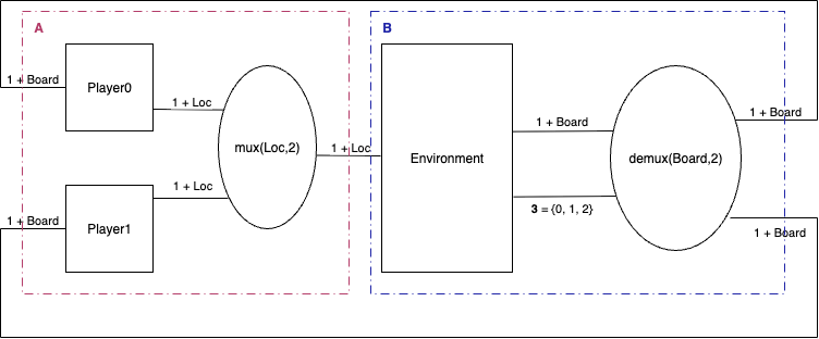
The dynamical system underlying our tic-tac-toe game stepper is then depicted as follows:

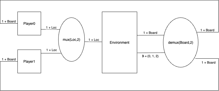
It contains three yet undefined stateful subsystems: \(\mathit{Player0}\), \(\mathit{Player1}\), and \(\mathit{Environment}\). Intuitively, the game stepper advances in a periodic pattern consisting of steps of four types, in order:

• \(\mathit{Environment}\) receives a move from \(\mathit{Player0}\) and executes its move
• \(\mathit{Environment}\) submits the resulting board to \(\mathit{Player1}\)
• \(\mathit{Environment}\) receives a move from \(\mathit{Player1}\) and executes its move
• \(\mathit{Environment}\) submits the resulting board to \(\mathit{Player0}\)

In sets of the form \(1 + X\), the \(1\) component on the left is typically used to mean “inactive”. For example, on turns in which \(\mathit{Player0}\) submits its move, and on turns in which the environment submits the board to a player, \(\mathit{Player1}\) outputs \((0,\ast)\). Likewise, when \(\mathit{Environment}\) submits a board to \(\mathit{Player0}\), the demultiplexor outputs \((0, \ast)\) along the bottom channel leading to \(\mathit{Player1}\).

Note that players can submit any location to the environment as a move. However, if the cell at the submitted location is already occupied with either \(0\) or \(1\), then the \(\mathit{Environment}\) will choose not to perform the action and advance control to the next player without changing the board.

Environment

We now define the \(\mathit{Environment}\) dynamical system. Our first task is deciding its set \(\mathit{State}_{\mathit{Environment}}\) of states. First, each state should convey the current execution step type

The \(\mathit{IllegalState}\) element above should be used when \(\mathit{Environment}\) receives an invalid input combination (i.e. one which we have prevented it from receiving by design). For those familiar with digital logic, this is somewhat analogous to a “don’t care” value.

Additionally, the state should convey the current board. We’ve already defined the set \(\mathit{Board}\) of board states above. Hence, our full state set is defined as

As figure 11 shows, the environment’s output set is

The environment’s \(\mathit{output}_\mathit{Environment} : \mathit{State}_{\mathit{Environment}} \to \mathit{Out}_{\mathit{Environment}}\) function is then defined as

Consulting figure 11, we see that

For \(b \in \mathit{Board}\), we define \(b[\ell \mapsto n] \in \mathit{Board}\) as follows.

We define \(\mathit{nextState}_{\mathit{Environment}} : \mathit{In}_{\mathit{Environment}} \times \mathit{State}_{\mathit{Environment}} \to \mathit{State}_{\mathit{Environment}}\) as \(~\\\) \(\mathit{nextState}_{\mathit{Environment}} : (1 + \mathit{Loc}) \times \mathit{StepType} \times \mathit{Board} \to \mathit{StepType} \times \mathit{Board}\) \(\mathit{nextState}_{\mathit{Environment}}((1,\ell), ReceiveFrom(n), b) \defeq \begin{cases} (SubmitTo((n+1)~\%~2), b[\ell \mapsto n]) & \text{if } b(\ell) = \_ \\ (SubmitTo((n+1)~\%~2), b) & \text{otherwise} \end{cases}\) \(\mathit{nextState}_{\mathit{Environment}}((0,\ast), SubmitTo(n), b) \defeq (ReceiveFrom(n), b)\)

and for any other \((z,s,b) \in (1 + Loc) \times \mathit{StepType} \times Board\) we define \(\mathit{nextState}_{\mathit{Environment}}(z,s,b) \defeq (\mathit{IllegalState}, b)\)

Finally, we define

Players

We define \(\mathit{Player0}\), eliding \(\mathit{Player1}\) as it is essentialy the same.

The state of the player systems can be used for two purposes. First, the state must record a \(Board\) whenever it is received from the environment. That way the player can use the board to compute a move on the next turn. Second, and optionally, a player’s state can serve as its brain by storing information about plan or strategy that the player is currently executing, or by storing an inferred mental model of the opposing player. We will keep things simple and decide moves in a stateless fashion, using only the current state of the board. Hence, we define

If the player’s state is \((1, b)\) then it has just received board \(b\) from the environment and is expected to submit a move on the next turn. Otherwise, the player’s state is \((0,\ast)\).

We can see from Diagram 11 that

and

Let \(\phi : \mathit{Board} \to \mathit{Loc}\) be player 0’s “strategy” for deciding a move given the current board; instead of defining it, we leave it as a parameter to the system.

We then define

and

The \(\mathit{Player0}\) dynamical system is then defined as

Putting things together

Now that all of the components of our system have been defined, we will wire them together using the lens composition technique, expressing the system as a whole as a mathematical expression.

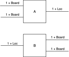
As a first step, we note that our system can be obtained by wiring together the two dynamical systems named \(A\) and \(B\) displayed below.

Where

and

Next, we take their parallel product \(A \otimes B\), which is depicted below.

Finally, to close off our system, we must wire together the two components using lens composition, similar to how we wired together the \(\mathit{Clock}\) and \(\mathit{Meridiem}\) systems above.

We use the wiring lens

where

and

Our complete system is then equal to:

Conclusion

Evaluating the Dynamical Systems Formalism

It’s worth taking a step back to ask whether the lens-based dynamical systems formalism is an appropriate tool for modelling turn-based computer games. The ability of lenses to represent cyclic data flow, from the players to the environment and back to the players, is essential. Additionally, lens based dynamical systems make it easy for us to encapsulate data, restricting a players to mutate only their own mental state, and restricting the environment to only mutate the physical world.

One drawback is that, due to the inherently concurrent nature of lens-based dynamical systems, we’ve needed to insert machinery for synchronization, which has little to do with dynamics of our turn-based games. For example, giving most wires the type \(1 + X\) is a distraction.

Looking ahead

Now that we’ve developed a mathematical model of a game stepper for tic-tac-toe, let’s recall the significant features listed at the end of my previous post and consider how well the model implements these features.

• ✅ A robot performs physical actions by submitting requests to an environment. The environment decides whether to honor these requests.
• ✅ A robot has internal state, but it’s a purely “mental” state that is used to make decisions. Physical properties of the robot are stored in the environment’s internal state.
• ❌ A robot may send a message to another robot, which represents information sent along some physical communication medium.

Our model implements the first two features. The game board can be seen as the environment, which encapsulates all physical information, namely the contents of every cell on the game board. A player can be seen as a robot; by virtue of being a dynamical systems, it encapsulates its own private data, i.e. mental state.

The last feature, message passing among robots, is not present in the model I described. Speculating, in a game’s source code, message passing might look similar to the following pseudo-code.

// When the player switches off the fuse box, this channel notifies all subscribers.
channel fuse_box_off : 1;

robot roy {
  receives on fuse_box_off;

  state working {
    handler fuse_box_off (_ : 1) = {
      set_state(fix_fusebox);
    }
  }

  state fix_fusebox {
    ...
  }
}

robot fuse_box {
  sends on fuse_box_off;

  state on {
    handler on_player_touch (_ : 1) = {
      send fuse_box_off(*);
      set_state(off);
    }
  }

  state off {
    ...
  }
}

Our program starts with a list of channel declarations. A channel declaration includes both a name and the type of messages sent along the channel. In this example, our channel is named fuse_box_off and has type \(1\), where \(1\) is the type of containing a single information-free value \(\ast\).

Each robot is implemented as a state machine. A robot definition begins with a list of declarations stating which channels the robot may send and receive upon. Next, the robot defines a list of states. These states can declare handlers to provide code that executes when a message is received, and the handlers in turn can issue send commands, which broadcast values to all of the subscribers of a channel.

If a robot sends a message along a channel, when is the message received by the channel’s subscribers? Our answer is that it is received on the next frame. The reason for this is that all robots acting on a frame are assumed to be acting at roughly the same time: times so close together that their difference is considered too fine-grained for our game engine to track.

A game engine may very reasonably execute multiple robot scripts in sequence on a single frame, but having the second robot receive messages sent by the first robot on the same frame is problematic. Not only does it violate our intuition that all robots are executing “at the same time” on a single frame, but it creates a hidden rule where a message sent from one robot to another may or may not arrive until the next frame depending on which robot was processed first.

If two robots transmit messages along the same channel on the same frame, which message do the channel’s subscribers process first? Since both messages are considered to be sent “at the same time,” our game system is too coarse-grained to answer this question. Our model should therefore non-deterministically permit any ordering. However, our current dynamical system formalism doesn’t support non-determinism.

The next blog post will correct this by extending the formalism with non-deterministic state transitions. It will also present a basic model of MegaZeux where all robots operate concurrently at every frame. We won’t have time to model message channels in that post, but by introducing non-determinism into the MegaZeux model, we will establish the foundation needed to add message passing in a subsequent post.

Next: Modelling MegaZeux